Chapter 6 Publication style figures and saving

‘ggpubr’ package is wondeful to create publication quality figures

diamonds2<-diamonds
levels(diamonds2$color)

## [1] "D" "E" "F" "G" "H" "I" "J"

diamonds2$color<- factor(diamonds2$color, levels =c("D" ,"E" ,"F" ,"G", "H", "I", "J"), 
                         labels=c("Red","Blue","Orange","Pink","Indigo","Jade","Orange"))
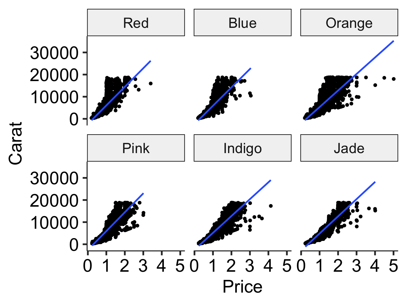
         ggplot(diamonds2)+
          geom_point(aes(x=carat,y=price))+
  geom_smooth(aes(x=carat,y=price),method='lm')+
  facet_wrap(~color)+
  ggpubr::theme_pubr(base_size=22)+
           
  ylab("Carat")+ xlab("Price")

## `geom_smooth()` using formula 'y ~ x'

Figure 6.1: Scatter plot with facets pub quality

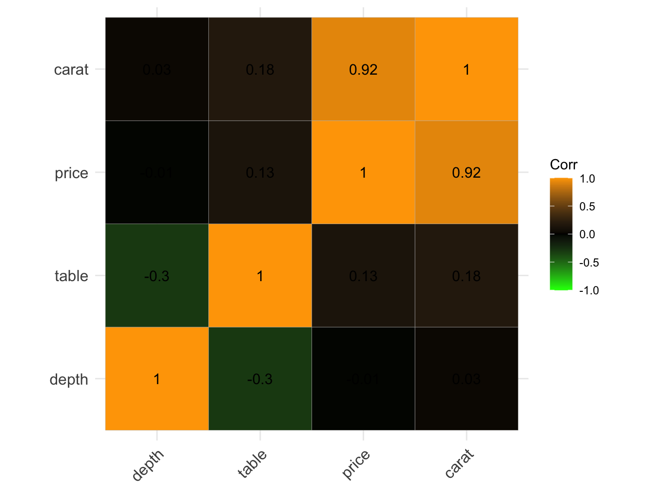
##Correlation plot

diamonds2<-diamonds %>% select(depth,table, price,carat)

# calulate the correlations
c <- cor(diamonds2, use="complete.obs")

library(ggcorrplot)
ggcorrplot(c,lab=T, color=c("green","black","orange"))

Figure 6.2: Correlation plot

6.1 Time series

Data collected in successive time points- dates, years, hours Let’s look at some time series data

Customize dates Weekday name: %a and %A for abbreviated and full weekday name, respectively Month name: %b and %B for abbreviated and full month name, respectively %d: day of the month as decimal number %U: week of the year as decimal number (00–53) %Y: Year

#tidyr::population
head(economics_long)

## # A tibble: 6 x 4
##   date       variable value  value01
##   <date>     <chr>    <dbl>    <dbl>
## 1 1967-07-01 pce       507. 0       
## 2 1967-08-01 pce       510. 0.000265
## 3 1967-09-01 pce       516. 0.000762
## 4 1967-10-01 pce       512. 0.000471
## 5 1967-11-01 pce       517. 0.000916
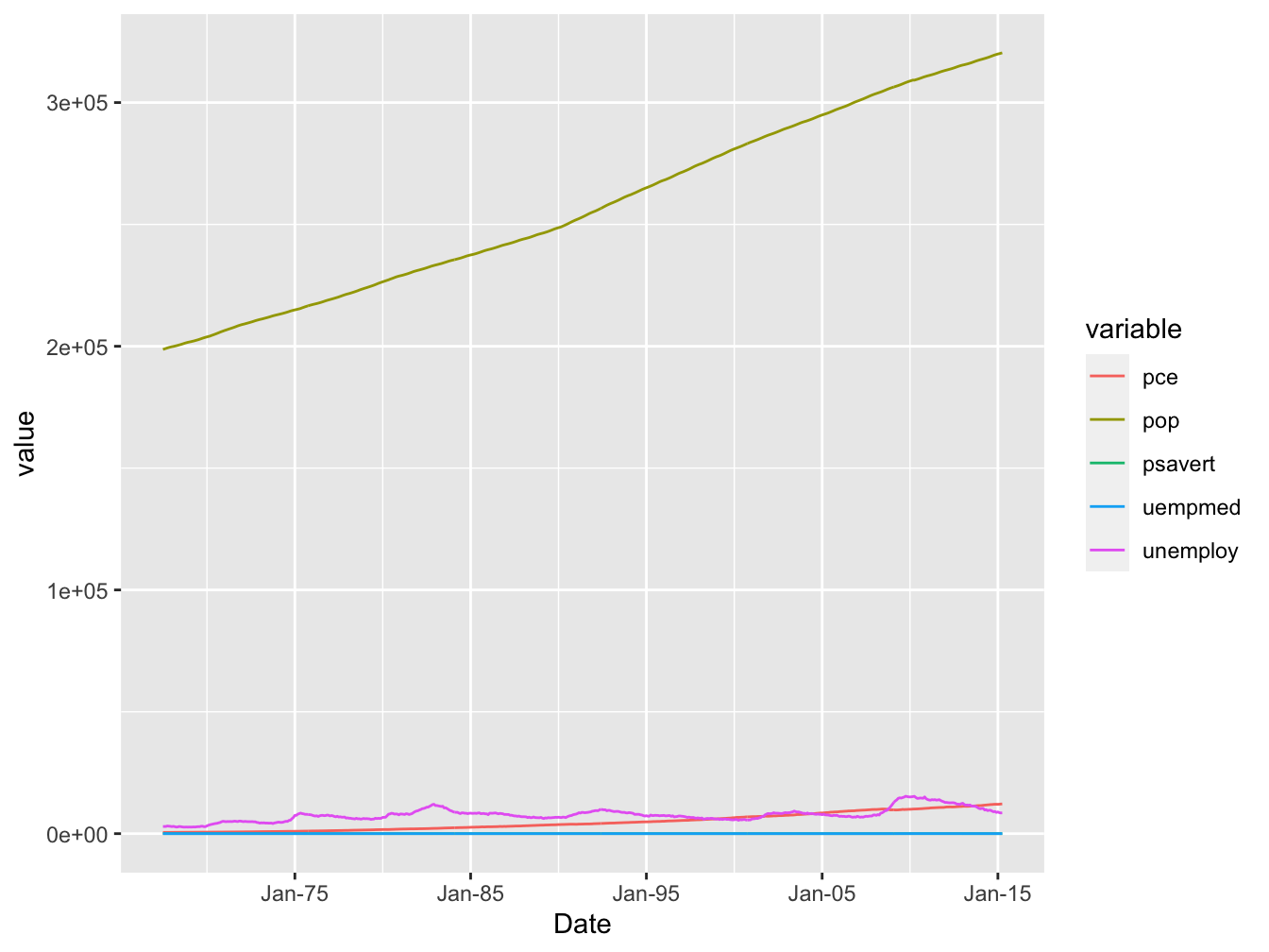
## 6 1967-12-01 pce       525. 0.00157

ggplot(economics_long)+
  geom_line(aes(date, value, color=variable))+
 scale_x_date(breaks='10 years',date_labels = "%b-%y")+ 
  xlab("Date")

Figure 6.3: time series plot